What is Cointegration?
A cointegration test is used to establish if there is a correlation between several time series in the long term. The concept was first introduced by Nobel laureates Robert Engle and Clive Granger in 1987 after British economist Paul Newbold and Granger published the spurious regression concept.
Cointegration tests identify scenarios where two or more non-stationary time series are integrated together in a way that they cannot deviate from equilibrium in the long term. The tests are used to identify the degree of sensitivity of two variables to the same average price over a specified period of time.
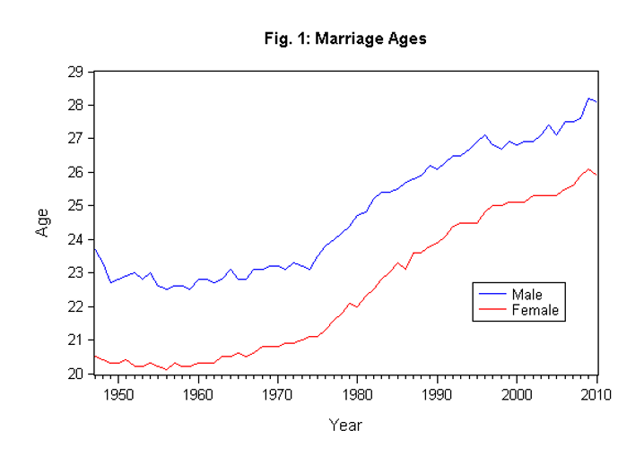
Cointegration of Gender as an Indicator of Marriage Age

Summary
- Cointegration is a technique used to find a possible correlation between time series processes in the long term.
- Nobel laureates Robert Engle and Clive Granger introduced the concept of cointegration in 1987.
- The most popular cointegration tests include Engle-Granger, the Johansen Test, and the Phillips-Ouliaris test.
History of Cointegration
Before the introduction of cointegration tests, economists relied on linear regressions to find the relationship between several time series processes. However, Granger and Newbold argued that linear regression was an incorrect approach for analyzing time series due to the possibility of producing a spurious correlation.
A spurious correlation occurs when two or more associated variables are deemed causally related due to either a coincidence or an unknown third factor. A possible result is a misleading statistical relationship between several time series variables.
Granger and Engle published a paper in 1987 in which they formalized the cointegrating vector approach. Their concept established that two or more non-stationary times series data are integrated together in a way that they cannot move away from some equilibrium in the long term.
The two economists argued against the use of linear regression to analyze the relationship between several time series variables because detrending would not solve the issue of spurious correlation. Instead, they recommended checking for cointegration of the non-stationary time series. They argued that two or more time series variables with I(1) trends could be cointegrated if it could be proved that there is a relationship between the variables.
Methods of Testing for Cointegration
There are three main methods of testing for cointegration. They are used to identify the long-term relationships between two or more sets of variables. The methods include:
1. Engle-Granger Two-Step Method
The Engle-Granger Two-Step method starts by creating residuals based on the static regression and then testing the residuals for the presence of unit-roots. It uses the Augmented Dickey-Fuller Test (ADF) or other tests to test for stationarity units in time series. If the time series is cointegrated, the Engle-Granger method will show the stationarity of the residuals.
The limitation of the Engle-Granger method is that if there are more than two variables, the method may show more than two cointegrating relationships. Another limitation is that it is a single equation model. However, some of the drawbacks have been addressed in recent cointegration tests like Johansen’s and Phillips-Ouliaris tests. The Engle-Granger test can be determined using STAT or MATLAB software
Consult a Data Analyst
We are a team of dedicated data analysts and econometricians that have competent experience in data modelling, statistical tests, hypothesis testing, predictive analysis and interpretation
- admin@datapott.com
2. Johansen Test
The Johansen test is used to test cointegrating relationships between several non-stationary time series data. Compared to the Engle-Granger test, the Johansen test allows for more than one cointegrating relationship. However, it is subject to asymptotic properties (large sample size) since a small sample size would produce unreliable results. Using the test to find cointegration of several time series avoids the issues created when errors are carried forward to the next step.
Johansen’s test comes in two main forms, i.e., Trace tests and Maximum Eigenvalue test.
- Trace tests
Trace tests evaluate the number of linear combinations in a time series data, i.e., K to be equal to the value K0, and the hypothesis for the value K to be greater than K0. It is illustrated as follows:
H0: K = K0
H0: K > K0
When using the trace test to test for cointegration in a sample, we set K0 to zero to test whether the null hypothesis will be rejected. If it is rejected, we can deduce that there exists a cointegration relationship in the sample. Therefore, the null hypothesis should be rejected to confirm the existence of a cointegration relationship in the sample.
- Maximum Eigenvalue test
An Eigenvalue is defined as a non-zero vector which, when a linear transformation is applied to it, changes by a scalar factor. The Maximum Eigenvalue test is similar to the Johansen’s trace test. The key difference between the two is the null hypothesis.
H0: K = K0
H0: K = K0 + 1
In a scenario where K=K0 and the null hypothesis is rejected, it means that there is only one possible outcome of the variable to produce a stationary process. However, in a scenario where K0 = m-1 and the null hypothesis is rejected, it means that there are M possible linear combinations. Such a scenario is impossible unless the variables in the time series are stationary.

