Understanding Three-way Interaction in ANOVA

Today i will teach you in Understanding Three-way Interaction in ANOVA

Consider the three-way ANOVA, shown below, with a significant three-way interaction. There are 24 observations in this analysis. In this model a has two levels, b two levels and c has three levels. You will note the significant three-way interaction. Basically, a three-way interaction means that one, or more, two-way interactions differ across the levels of a third variable. In this page, we will show you the steps that are involved and work through them manually.

For the purposes of this example we are going to focus on the b*c interaction and how it changes across levels of a.

                  Source |  Partial SS    df       MS           F     Prob > F
              -----------+----------------------------------------------------
                       a |         150     1         150     112.50     0.0000
                       b |  .666666667     1  .666666667       0.50     0.4930
                       c |  127.583333     2  63.7916667      47.84     0.0000
                     a*b |  160.166667     1  160.166667     120.13     0.0000
                     a*c |       18.25     2       9.125       6.84     0.0104
                     b*c |  22.5833333     2  11.2916667       8.47     0.0051
                   a*b*c |  18.5833333     2  9.29166667       6.97     0.0098
                         |
                Residual |          16    12  1.33333333   
              -----------+----------------------------------------------------
                   Total |  513.833333    23  22.3405797

Image at_a_1 Image at_a_2

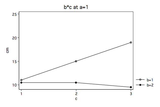
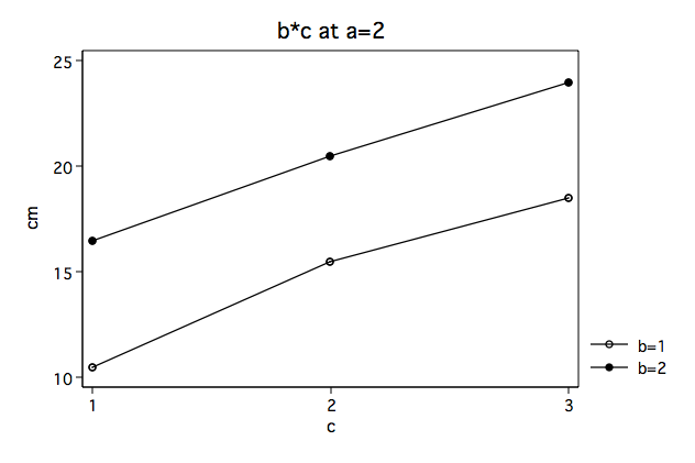
In looking at the plots (above) it appears that the b*c interaction looks very different at the two levels of a. We suspect that there is a significant interaction at a=1 but that the interaction is not significant at a=2. So we need to be able to provide some statistical evidence to back this suspicion up.

We will start by running an ANOVA with just b and c for those cases in which a=1.

                  Source |  Partial SS    df       MS           F     Prob > F
              -----------+----------------------------------------------------
                       b |  70.0833333     1  70.0833333      56.07     0.0003
                       c |  24.6666667     2  12.3333333       9.87     0.0127
                     b*c |  40.6666667     2  20.3333333      16.27     0.0038
                         |
                Residual |         7.5     6        1.25   
              -----------+----------------------------------------------------
                   Total |  142.916667    11  12.9924242

There is a problem in the above table. The F-ratio in the table is wrong. The reason that the F-ratio is wrong is that it uses the wrong error term (residual). It is using an error term based on just 6 degrees of freedom and not on the 12 degrees of freedom found in the original model. We should be using the mean square residual from the original three-factor model. We need to recompute the F-ratio using the the mean square residual equal to 1.33333333. Here is the correct computation for the F-ratio.

F(2, 12) = MS(b*c)/MS(residual) = 20.3333333/1.33333333 = 15.25

Next, we will repeat the process for a=2 including the manual computation of the F-ratio.

                  Source |  Partial SS    df       MS           F     Prob > F
              -----------+----------------------------------------------------
                       b |       90.75     1       90.75      64.06     0.0002
                       c |  121.166667     2  60.5833333      42.76     0.0003
                     b*c |          .5     2         .25       0.18     0.8424
                         |
                Residual |         8.5     6  1.41666667   
              -----------+----------------------------------------------------
                   Total |  220.916667    11  20.0833333 

F(2, 12) = MS(b*c)/MS(residual) = .25/1.33333333 = .1875

Need Help with Researchers or Data Analysts, Lets Help you with Data Analysis & Result Interpretation for your Project, Thesis or Dissertation?

We are Experts in SPSS, EVIEWS, AMOS, STATA, R, and Python

Clearly, one F-ratio is much larger than the other but how can we tell which are statistically significant? There are at least four different methods of determining the critical value of tests of this type. There is a method related to Dunn’s multiple comparisons, a method attributed to Marascuilo and Levin, a method called the simultaneous test procedure (very conservative and related to the Scheffé post-hoc test) and a per family error rate method. We will demonstrate the per family error rate method but you should look up the other methods in a good ANOVA book, like Kirk (1995), to decide which approach is best for your situation.

The per family error rate critical value for this example is approximately equal to 5.1. Using this critical value the first F-ratio of 15.25 is significant while the second (.1875) is not. In other words, the two-way b*c interaction is significant at a = 1 but is not significant at a = 2.

So now we know that there is a significant b*c interaction at a=1. This interaction also needs to be understood. We can do this by test the differences in the levels of c for each level of b still holding a=1.

                  Source |  Partial SS    df       MS           F     Prob > F
              -----------+----------------------------------------------------
                       c |          64     2          32      16.00     0.0251
                         |
                Residual |           6     3           2   
              -----------+----------------------------------------------------
                   Total |          70     5          14   

This model like the a*b interaction earlier uses the wrong error term. We will once again have to use the correct error term and compute the F-ratio manually.

F(2, 12) = MS(c)/MS(residual) = 32/1.33333333 = 24

Now, we repeat the process with b=2 including the computation of the F-ratio.

                  Source |  Partial SS    df       MS           F     Prob > F
              -----------+----------------------------------------------------
                       c |  1.33333333     2  .666666667       1.33     0.3852
                         |
                Residual |         1.5     3          .5   
              -----------+----------------------------------------------------
                   Total |  2.83333333     5  .566666667 

F(2, 12) = MS(c)/MS(residual) = .666666667/1.33333333 = .5

We will continue to use a critical value based on the per family error rate. The critical value with 2 and 12 degrees of freedom is about 5.1. With this critical value the effect of c at b=1 (holding a at 1) is significant while c at b=2 (holding a at 1) in not significant.

Since the effect of c at b=1 and a=1 is statistically significant and has more than two levels, we should follow this up with some type of pairwise comparisons. With real data we would do that but, for now, it is a topic for another page.

We can summarize the original ANOVA and all of the follow up tests into a single ANOVA summary table. Which looks something like this.

                  Source |  Partial SS    df       MS           F     Prob > F
              -----------+----------------------------------------------------
                       a |         150     1         150     112.50     0.0000
                       b |  .666666667     1  .666666667       0.50     0.4930
                       c |  127.583333     2  63.7916667      47.84     0.0000
                     a*b |  160.166667     1  160.166667     120.13     0.0000
                     a*c |       18.25     2       9.125       6.84     0.0104
                     b*c |  22.5833333     2  11.2916667       8.47     0.0051
                   a*b*c |  18.5833333     2  9.29166667       6.97     0.0098
                         |----------------------------------------------------
                 b*c @ a |
               b*c @ a=1 |  40.6666667     2  20.3333333      15.25     p<.05
               b*c @ a=2 |          .5     2         .25       0.19     n.s.
                         |----------------------------------------------------
             c @ b (a=1) |
             c @ b=1 a=1 |          64     2          32      24.00     p<.05
             c @ b=2 a=1 |  1.33333333     2  .666666667       0.50     n.s.
                         |
                Residual |          16    12  1.33333333   
              -----------+----------------------------------------------------
                   Total |  513.833333    23  22.3405797   

If you would like more details on how to implement these tests following a significant

Data Analytics Services
Need Our Services?
Econometrics & Statistics Modelling Services
Need Help, Whatsapp Us Now