Both are types of generalized linear models. This means they have this form:

Both can be used for modeling the relationship between one or more numerical or categorical predictor variables and a categorical outcome.

Both have versions for binary, ordinal, or multinomial categorical outcomes. And each of these requires specific coding of the outcome. For example, in both logistic and probit models, a binary outcome must be coded as 0 or 1.

So logistic and probit models can be used in the exact same situations. How do they differ?

The real difference is theoretical: they use different link functions.

In generalized linear models, instead of using Y as the outcome, we use a function of the mean of Y. This is the link function.

A logistic regression uses a logit link function:

And a probit regression uses an inverse normal link function:

These are not the only two link functions that can be used for categorical data, but they’re the most common.

Think about the binary case: Y can have only values of 1 or 0, and we’re really interested in how a predictor relates to the probability that Y=1. But we can’t use the probability itself as the function above. There are two big reasons:

1. Probability can only have values between 0 and 1, whereas the right hand side of the equation can vary from -∞ to ∞.

2. The relationship between probability and the predictors isn’t linear, it’s sigmoidal (a.k.a., S-shaped).

So we need a function of the probability that does two things: (1) converts a probability into a value that runs from -∞ to ∞ and (2) has a linear relationship with the Xs. Probit and Logistic functions both do that.

The difference in the overall results of the model are usually slight to non-existent, so on a practical level it doesn’t usually matter which one you use.

The choice usually comes down to interpretation and communication.

Interpretation:

Anyone who has ever struggled to interpret an odds ratio may find it difficult to believe that a logistic link leads to more intuitive coefficients. Because we can back transform those log-odds into odds ratios, we can get a somewhat intuitive way to interpret effects.

With a probit link, it’s not so easy. After all, what does that inverse normal really mean?

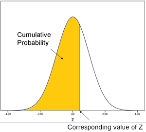
Remember back to intro stats when you had to look up in Z tables the area under the normal curve for a specific Z value? That area represents a cumulative probability: the probability that Z is less than or equal to the specified Z value.

When we do the inverse normal transformation, we’re going in the opposite direction: for any cumulative probability, what is the corresponding Z value?

(See how there is a direct conversion from a probability to a number line that runs from -∞ to ∞)?

So you can think of the probit function as the Z (standard normal) value that corresponds to a specific cumulative probability.

Coefficients for probit models can be interpreted as the difference in Z score associated with each one-unit difference in the predictor variable.

Not very intuitive.

Another way to interpret these coefficients is to use the model to calculate predicted probabilities at different values of X.

Remember, though, just like in logistic regression, the difference in the probability isn’t equal for each 1-unit change in the predictor. The sigmoidal relationship between a predictor and probability is nearly identical in probit and logistic regression. A 1-unit difference in X will have a bigger impact on probability in the middle than near 0 or 1.

That said, if you do enough of these, you can certainly get used the idea. Then you will start to have a better idea of the size of each Z-score difference.