We now show how to test the value of the slope of the regression line.

Basic Approach

By Property 1 of One Sample Hypothesis Testing for Correlation, under certain conditions, the test statistic t has the property

But by Property 1 of Method of Least Squares

and by Definition 3 of Regression Analysis and Property 4 of Regression Analysis

Putting these elements together we get that

where

Since by the population version of Property 1 of Method of Least Squares

it follows that ρ = 0 if and only if β = 0. Thus Theorem 1 of One Sample Hypothesis Testing for Correlation can be transformed into the following test of the hypothesis H₀: β = 0 (i.e. the slope of the population regression line is zero):

Example

Example 1: Test whether the slope of the regression line in Example 1 of Method of Least Squares is zero.

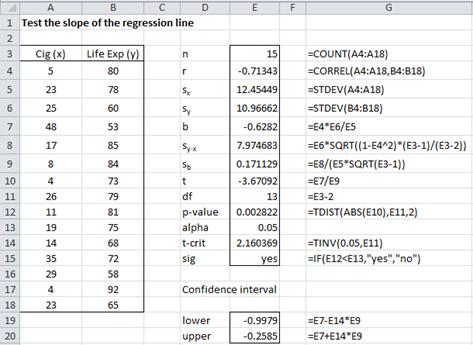
Figure 1 shows the worksheet for testing the null hypothesis that the slope of the regression line is 0.

Figure 1 – t-test of the slope of the regression line

Since p-value = .0028 < .05 = α (or |t| = 3.67 > 2.16 = t_crit) we reject the null hypothesis, and so we can’t conclude that the population slope is zero.

Note that the 95% confidence interval for the population slope is

b ± t_crit · s_b = -628 ± 2.16(.171) = (-.998, -.259)

Testing equality of slopes

We can also test whether the slopes of the regression lines arising from two independent populations are significantly different. This would be useful for example when testing whether the slope of the regression line for the population of men in Example 1 is significantly different from that of women.

Click here for additional information and an example about Hypothesis Testing for Comparing the Slopes of Two Independent Samples.

Worksheet Functions

Excel Functions: where R1 = the array of observed values and R2 = the array of observed values.

STEYX(R1, R2) = standard error of the estimate s_y∙x = SQRT(MS_Res)

LINEST(R1, R2, TRUE, TRUE) – an array function that generates a number of useful statistics.

To use LINEST, begin by highlighting a blank 5 × 2 range, enter =LINEST( and then highlight the R1 array, enter a comma, highlight the R2 array and finally enter ,TRUE,TRUE) and press Ctrl-Shft-Enter.

The LINEST function returns a number of values, but unfortunately no labels for these values. To make all of this clearer, Figure 2 displays the output from LINEST(A4:A18, B4:B18, TRUE, TRUE) using the data in Figure 1. I have added the appropriate labels manually for clarity.

Figure 2 – LINEST(B4:B18,A4:A18,TRUE,TRUE) output

R Square is the correlation of determination r² (see Definition 2 of Basic Concepts of Correlation), while all the other values are as described above with the exception of the standard error of the y-intercept, which will be explained shortly.

Data analysis tool

Excel also provides a Regression data analysis tool. The creation of a regression line and hypothesis testing of the type described in this section can be carried out using this tool. Figure 3 displays the principal output of this tool for the data in Example 1.

Figure 3 – Output from Regression data analysis tool

The following is a description of the fields in this report:

Summary Output

• Multiple R – correlation coefficient (see Definition 1 of Multiple Correlation, although since there is only one independent variable this is equivalent to Definition 2 of Basic Concepts of Correlation)
• R Square – coefficient of determination (see Definition 1 of Multiple Correlation), i.e. the square of Multiple R
• Adjusted R Square – see Definition 2 of Multiple Correlation
• Standard Error = SQRT(MS_Res), can also be calculated using Excel’s STEYX function
• Observations – sample size

ANOVA

• The first row lists the values for df_Reg, SS_Reg, MS_Reg, F = MS_Reg/MS_Res and p-value
• The second row lists the values for df_Res, SS_Res and MS_Res
• The third row lists the values for df_T and SS_T

Coefficients (third table)

The third table gives key statistics for testing the y-intercept (Intercept in the table) and slope (Cig in the table). We will explain the intercept statistics in Confidence and Prediction Intervals for Forecasted Values. The slope statistics are as follows:

• Coefficients – value for the slope of the regression line
• Standard Error – standard error of the slope, s_b = s_y∙x / (ss_x * SQRT(n-1))
• t-Stat = b/s_b
• P-value = T.DIST.2T(t, df_Res); i.e. 2-tailed value; =TDIST(t, df_Res, 2) in Excel 2007
• 95% confidence interval = b ± t_crit ∙ s_b

Residuals

In addition to the principal results described in Figure 3, one can optionally generate a table of residuals and a table of percentiles as described in Figure 4.

Figure 4 – Additional output from Regression data analysis tool

Residual Output:

• Predicted Life Exp = Cig * b + a; i.e. ŷ
• Residuals = Observed Life Exp – Predicted Life Exp; i.e. y – ŷ
• Standard Residuals = Residual / Std Dev of the Residuals (since the mean of the residuals is expected to be 0): i.e. e/s_e

For example. for Observation 1 we have

• Predicted Life Exp = -.63 * 5 + 85.72 = 82.58
• Residuals = 80 – 82.58 = -2.58
• Standard Residuals = -2.58 / 7.69 = -.336

Note that the mean of the residuals is approximately 0 (which is consistent with a key assumption of the regression model) and a standard deviation of 7.69.

There is also the option to produce certain charts, which we review when discussing Example 2 of Multiple Regression Analysis.