Normality
Normality refers to the distribution of the data for a particular variable. We usually assume that the data is normally distributed, even though it usually is not! Normality is assessed in many different ways: shape, skewness, and kurtosis (flat/peaked).
- Shape: To discover the shape of the distribution in SPSS, build a histogram (as shown in the video tutorial) and plot the normal curve. If the histogram does not match the normal curve, then you likely have normality issues. You can also look at the boxplot to determine normality.
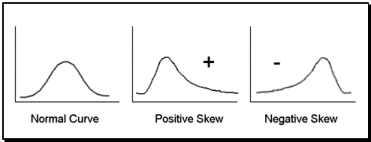
- Skewness: Skewness means that the responses did not fall into a normal distribution, but were heavily weighted toward one end of the scale. Income is an example of a commonly right skewed variable; most people make between 20 and 70 thousand dollars in the USA, but there is smaller group that makes between 70 and 100, and an even smaller group that makes between 100 and 150, and a much smaller group that makes between 150 and 250, etc. all the way up to Bill Gates and Mark Zuckerberg. Addressing skewness may require transformations of your data (if continuous), or removing influential outliers. There are two rules on Skewness:
- (1)If your skewness value is greater than 1 then you are positive (right) skewed, if it is less than -1 you are negative (left) skewed, if it is in between, then you are fine. Some published thresholds are a bit more liberal and allow for up to +/-2.2, instead of +/-1.
- (2)If the absolute value of the skewness is less than three times the standard error, then you are fine; otherwise you are skewed.
Using these rules, we can see from the table below, that all three variables are fine using the first rule, but using the second rule, they are all negative (left) skewed.
Need Help with Data Analysis & Result Interpratation for your Project, Thesis or Dissertation?
We are Experts in SPSS, EVIEWS, AMOS, STATA, R, and Python
Skewness looks like this:
- Kurtosis:
Kurtosis refers to the outliers of the distribution of data. Data that have outliers have large kurtosis. Data without outliers have low kurtosis. The kurtosis (excess kurtosis) of the normal distribution is 0. The rule for evaluating whether or not your kurtosis is problematic is the same as rule two above:
- If the absolute value of the kurtosis is less than three times the standard error, then the kurtosis is not significantly different from that of the normal distribution; otherwise you have kurtosis issues. Although a looser rule is an overall kurtosis score of 2.200 or less (rather than 1.00) (Sposito et al., 1983).
Kurtosis looks like this:
- Bimodal:
One other issue you may run into with the distribution of your data is a bimodal distribution. This means that the data has multiple (two) peaks, rather than peaking at the mean. This may indicate there are moderating variables effecting this data. A bimodal distribution looks like this:
- Transformations
When you have extremely non-normal data, it will influence your regressions in SPSS and AMOS. In such cases, if you have non-Likert-scale variables (so, variables like age, income, revenue, etc.), you can transform them prior to including them in your model. Gary Templeton has published an excellent article on this and created a YouTube video showing how to conduct the transformation. He also references his article in the video.


