Linear vs. Logistic Probability Models: Which is Better, and When?

Interpretability

Let’s start by comparing the two models explicitly. If the outcome Y is a dichotomy with values 1 and 0, define p = E(Y|X), which is just the probability that Y is 1, given some value of the regressors X. Then the linear and logistic probability models are:

p = a+ a1X1 + a2X2 + … + akXk    (linear)

ln[p/(1-p)] = b+ b1X1 + b2X2 + … + bkXk       (logistic)

The linear model assumes that the probability p is a linear function of the regressors, while the logistic model assumes that the natural log of the odds p/(1-p) is a linear function of the regressors.

The major advantage of the linear model is its interpretability. In the linear model, if a1 is (say) .05, that means that a one-unit increase in X1 is associated with a 5 percentage point increase in the probability that Y is 1. Just about everyone has some understanding of what it would mean to increase by 5 percentage points their probability of, say, voting, or dying, or becoming obese.

The logistic model is less interpretable. In the logistic model, if b1 is .05, that means that a one-unit increase in X1 is associated with a .05 increase in the log odds that Y is 1. And what does that mean? I’ve never met anyone with any intuition for log odds.

How intuitive are odds ratios?

Because the log odds scale is so hard to interpret, it is common to report logistic regression results as odds ratios. To do this, we exponentiate both sides of the logistic regression equation and obtain a new equation that looks like this:

p/(1-p) = d0 × (d1)X1 × (d2)X2 × … × (dk)Xk

On the left side we have the odds and on the right side we have a product involving the odds ratios d= exp(b1), d2 = exp(b2), etc.

Odds ratios seem like they should be intuitive. If d1 = 2, for example, that means that a one-unit increase in Xdoubles the odds that Y is 1. That sounds like something we should understand.

But we don’t understand, really. We think we understand odds because in everyday speech we use the word “odds” in a vague and informal way. Journalists commonly use “odds” interchangeably with a variety of other words, such as “chance,” “risk,” “probability,” and “likelihood”—and academics are often just as sloppy when interpreting results. But in statistics these words aren’t synonyms. The word odds has a very specific meaning—p/(1-p)—and so does the odds ratio.

Still think you have an intuition for odds ratios? Let me ask you a question. Suppose a get-out-the-vote campaign can double your odds of voting. If your probability of voting was 40% before the campaign, what is it after? 80%? No, it’s 57%.

If you got that wrong, don’t feel bad. You’ve got a lot of company. And if you got it right, I bet you had to do some mental arithmetic[1], or even use a calculator, before answering. The need for arithmetic should tell you that odds ratios aren’t intuitive.

Here’s a table that shows what doubling the odds does to various initial probabilities:

Before doublingAfter doubling
ProbabilityOddsOddsProbability
10%0.110.2218%
20%0.250.5033%
30%0.430.8646%
40%0.671.3357%
50%1.002.0067%
60%1.503.0075%
70%2.334.6782%
80%4.008.0089%
90%9.0018.095%

It isn’t simple. The closest I’ve come to developing an intuition for odds ratios is this: If p is close to 0, then doubling the odds is approximately the same as doubling p. If p is close to 1, then doubling the odds is approximately the same as halving 1-p. But if p is in the middle—not too close to 0 or 1—then I don’t really have much intuition and have to resort to arithmetic.

That’s why I’m not crazy about odds ratios.


Stuck with Your Research or Data Analysis Project?

Let Our Experts Help You

How nonlinear is the logistic model?

The logistic model is unavoidable if it fits the data much better than the linear model. And sometimes it does. But in many situations the linear model fits just as well, or almost as well, as the logistic model. In fact, in many situations, the linear and logistic model give results that are practically indistinguishable except that the logistic estimates are harder to interpret (Hellevik 2007).

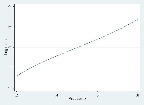
For the logistic model to fit better than the linear model, it must be the case that the log odds are a linear function of X, but the probability is not. And for that to be true, the relationship between the probability and the log odds must itself be nonlinear. But how nonlinear is the relationship between probability and log odds? If the probability is between .20 and .80, then the log odds are almost a linear function of the probability  (cf. Long 1997).

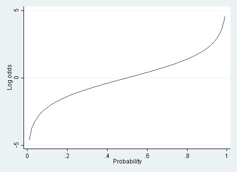
It’s only when you have a really wide range of probabilities—say .01 to .99—that the linear approximation totally breaks down.

When the true probabilities are extreme, the linear model can also yield predicted probabilities that are greater than 1 or less than 0. Those out-of-bounds predicted probabilities are the Achilles heel of the linear model.

A rule of thumb

These considerations suggest a rule of thumb. If the probabilities that you’re modeling are extreme—close to 0 or 1—then you probably have to use logistic regression. But if the probabilities are more moderate—say between .20 and .80, or a little beyond—then the linear and logistic models fit about equally well, and the linear model should be favored for its ease of interpretation.

Both situations occur with some frequency. If you’re modeling the probability of voting, or of being overweight, then nearly all the modeled probabilities will be between .20 and .80, and a linear probability model should fit nicely and offer a straightforward interpretation. On the other hand, if you’re modeling the probability that a bank transaction is fraudulent—as I used to do—then the modeled probabilities typically range between .000001 and .20. In that situation, the linear model just isn’t viable, and you have to use a logistic model or another nonlinear model (such as a neural net).

Keep in mind that the logistic model has problems of its own when probabilities get extreme. The log odds ln[p/(1-p)] are undefined when p is equal to 0 or 1. When p gets close to 0 or 1 logistic regression can suffer from complete separation, quasi-complete separation, and rare events bias (King & Zeng, 2001). These problems are less likely to occur in large samples, but they occur frequently in small ones. Users should be aware of available remedies. See Paul Allison’s post on this topic.

Computation and estimation

Interpretability is not the only advantage of the linear probability model. Another advantage is computing speed. Fitting a logistic model is inherently slower because the model is fit by an iterative process of maximum likelihood. The slowness of logistic regression isn’t noticeable if you are fitting a simple model to a small or moderate-sized dataset. But if you are fitting a very complicated model or a very large data set, logistic regression can be frustratingly slow.

The linear probability model is fast by comparison because it can be estimated noniteratively using ordinary least squares (OLS). OLS ignores the fact that the linear probability model is heteroskedastic with residual variance p(1-p), but the heteroscedasticity is minor if p is between .20 and .80, which is the situation where I recommend using the linear probability model at all. OLS estimates can be improved by using heteroscedasticity-consistent standard errors or weighted least squares. In my experience these improvements make little difference, but they are quick and reassuring.

Data Analytics Services
Need Our Services?
Econometrics & Statistics Modelling Services
Need Help, Whatsapp Us Now