This article explains how to perform point forecasting in STATA, where one can generate forecast values even without performing ARIMA. Therefore, it is useful in any time series data.

Forecasting is an important part of time series analysis. A point forecast is a singular number which represents the estimate of the true but unknown value of a variable at a future date. The data on Gross Domestic Product (GDP), Gross Fixed Capital Formation (GFC) and Private Capital Consumption (PFC) for the same time period (1997 to 2017) as considered in the previous article is used.

Performing point forecasting in STATA

Step 1: Declare data as time series

The first step is to declare the data to be time series. For this, follow the below steps.

Stata command:

This will arrange the time series data as follows.

In the figure above, the last observation is 2017. To use point forecasting, extend the data for some more years depending on which forecast values are needed using ‘tsappend’ command.

tsappend, add(3)
tsappend, last (2020Q4) tsfmt(tq)

This command will add time period until 2020.Alternatively, use the following command.

Observations up to 2017 are ‘in-sample’ observations whereas observations after 2017 are ‘out of the sample’ observations (figure above).

Step 2: Use regression coefficients

Then use the regression coefficients with the following command.

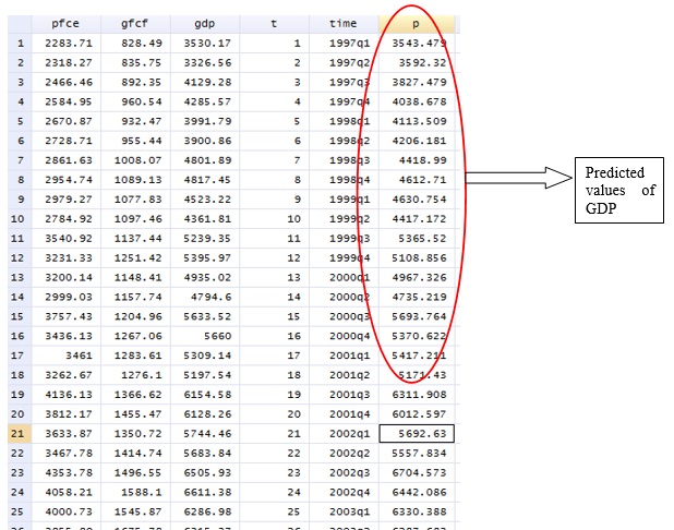
regress gdp gfcf pfce

After the regression, use the ‘predict’ command for point forecasting, so long as the regressors are available. ‘p’ is any new variable representing GDP (since GDP is the dependent variable in the regression model). Step 3: Use the ‘predict’ command.

predict p

In-sample and out of sample data: The command ‘predict p’ will generate forecast values for in sample observations and out-of-sample observations.

To restrict the forecasting to be in‐sample (for quarterly data), use the following command.

predict p if t<=tq(2017q4)
predict yp if t>tq(2017q4)

For the out of sample (for quarterly data) prediction use the following command. This command will give forecast values of gdp, (here in p variable) in the data set (figure below).

To plot GDP and ‘p’ in graph, use the following command.

tsline gdp p

The figure below will appear.

The figure above represents the actual values and forecast values of GDP (p variable). The figure shows that there is a very slight difference actual GDP and forecast GDP values. It implies that in this case, point forecasting can effectively generate forecasted values of GDP for any time period in future.

Shortcomings of point forecasting

In point forecasting, the prediction is possible at each specific point of the data series. However, one criticism of point forecasting is that it does not provide the degree of uncertainty that is associated with the forecast. To take into account variability in forecasting, interval forecasting is applicable as an alternative to point forecasting.