How to conduct Linear regression analysis using Stata

Example

Studies show that exercising can help prevent heart disease. Within reasonable limits, the more you exercise, the less risk you have of suffering from heart disease. One way in which exercise reduces your risk of suffering from heart disease is by reducing a fat in your blood, called cholesterol. The more you exercise, the lower your cholesterol concentration. Furthermore, it has recently been shown that the amount of time you spend watching TV – an indicator of a sedentary lifestyle – might be a good predictor of heart disease (i.e., that is, the more TV you watch, the greater your risk of heart disease).

Therefore, a researcher decided to determine if cholesterol concentration was related to time spent watching TV in otherwise healthy 45 to 65 year old men (an at-risk category of people). For example, as people spent more time watching TV, did their cholesterol concentration also increase (a positive relationship); or did the opposite happen? The researcher also wanted to know the proportion of cholesterol concentration that time spent watching TV could explain, as well as being able to predict cholesterol concentration. The researcher could then determine whether, for example, people that spent eight hours spent watching TV per day had dangerously high levels of cholesterol concentration compared to people watching just two hours of TV.

To carry out the analysis, the researcher recruited 100 healthy male participants between the ages of 45 and 65 years old. The amount of time spent watching TV (i.e., the independent variable, time_tv) and cholesterol concentration (i.e., the dependent variable, cholesterol) were recorded for all 100 participants. Expressed in variable terms, the researcher wanted to regress cholesterol on time_tv.

Note: The example and data used for this guide are fictitious. We have just created them for the purposes of this guide.

Stata

Setup in Stata

In Stata, we created two variables: (1) time_tv, which is the average daily time spent watching TV in minutes (i.e., the independent variable); and (2) cholesterol, which is the cholesterol concentration in mmol/L (i.e., the dependent variable).

Note: It does not matter whether you create the dependent or independent variable first.

After creating these two variables – time_tv and cholesterol – we entered the scores for each into the two columns of the Data Editor (Edit) spreadsheet (i.e., the time in hours that the participants watched TV in the left-hand column (i.e., time_tv, the independent variable), and participants’ cholesterol concentration in mmol/L in the right-hand column (i.e., cholesterol, the dependent variable), as shown below: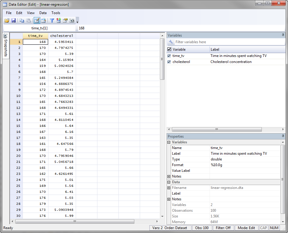

Published with written permission from StataCorp LP.

Stata

Test Procedure in Stata

In this section, we show you how to analyse your data using linear regression in Stata when the six assumptions in the previous section, Assumptions, have not been violated. You can carry out linear regression using code or Stata’s graphical user interface (GUI). After you have carried out your analysis, we show you how to interpret your results. First, choose whether you want to use code or Stata’s graphical user interface (GUI).

Code

The code to carry out linear regression on your data takes the form:

regress DependentVariable IndependentVariable

This code is entered into the  box below:

Published with written permission from StataCorp LP.

Using our example where the dependent variable is cholesterol and the independent variable is time_tv, the required code would be:

regress cholesterol time_tv

Note 1: You need to be precise when entering the code into the  box. The code is “case sensitive”. For example, if you entered “Cholesterol” where the “C” is uppercase rather than lowercase (i.e., a small “c”), which it should be, you will get an error message like the following:

Note 2: If you’re still getting the error message in Note 2: above, it is worth checking the name you gave your two variables in the Data Editor when you set up your file (i.e., see the Data Editor screen above). In the  box on the right-hand side of the Data Editor screen, it is the way that you spelt your variables in the  section, not the  section that you need to enter into the code (see below for our dependent variable). This may seem obvious, but it is an error that is sometimes made, resulting in the error in Note 2 above.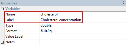

Therefore, enter the code, regress cholesterol time_tv, and press the “Return/Enter” button on your keyboard.

Published with written permission from StataCorp LP.

You can see the Stata output that will be produced here.

Graphical User Interface (GUI)

The three steps required to carry out linear regression in Stata 12 and 13 are shown below:

1. Click Statistics > Linear models and related > Linear regression on the main menu, as shown below: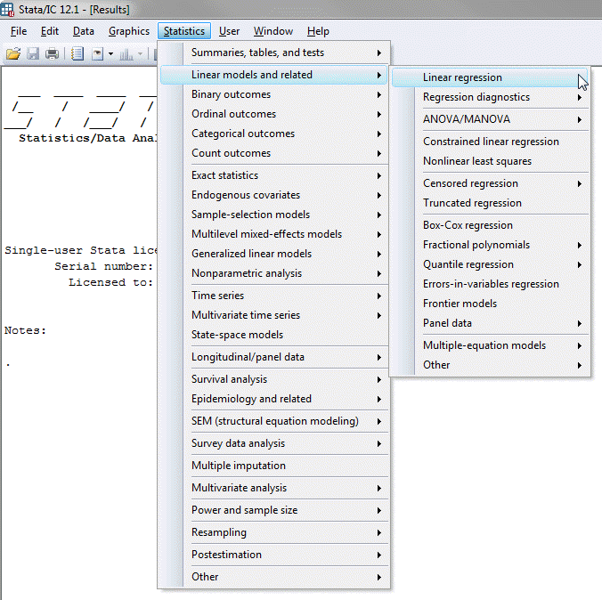Published with written permission from StataCorp LP.
   You will be presented with the Regress – Linear regression dialogue box: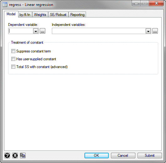
   Published with written permission from StataCorp LP.
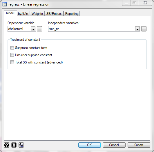
2. Select cholesterol from within the Dependent variable: drop-down box, and time_tv from within the Independent variables: drop-down box. You will end up with the following screen:Published with written permission from StataCorp LP.
3. Click on the  button. This will generate the output.

Stata

Output of linear regression analysis in Stata

If your data passed assumption #3 (i.e., there was a linear relationship between your two variables), #4 (i.e., there were no significant outliers), assumption #5 (i.e., you had independence of observations), assumption #6 (i.e., your data showed homoscedasticity) and assumption #7 (i.e., the residuals (errors) were approximately normally distributed), which we explained earlier in the Assumptions section, you will only need to interpret the following linear regression output in Stata: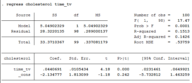

Published with written permission from StataCorp LP.

The output consists of four important pieces of information: (a) the R² value (“R-squared” row) represents the proportion of variance in the dependent variable that can be explained by our independent variable (technically it is the proportion of variation accounted for by the regression model above and beyond the mean model). However, R² is based on the sample and is a positively biased estimate of the proportion of the variance of the dependent variable accounted for by the regression model (i.e., it is too large); (b) an adjusted R² value (“Adj R-squared” row), which corrects positive bias to provide a value that would be expected in the population; (c) the F value, degrees of freedom (“F( 1, 98)“) and statistical significance of the regression model (“Prob > F” row); and (d) the coefficients for the constant and independent variable (“Coef.” column), which is the information you need to predict the dependent variable, cholesterol, using the independent variable, time_tv.

In this example, R² = 0.151. Adjusted R² = 0.143 (to 3 d.p.), which means that the independent variable, time_tv, explains 14.3% of the variability of the dependent variable, cholesterol, in the population. Adjusted R² is also an estimate of the effect size, which at 0.143 (14.3%), is indicative of a medium effect size, according to Cohen’s (1988) classification. However, normally it is R² not the adjusted R² that is reported in results. In this example, the regression model is statistically significant, F(1, 98) = 17.47, p = .0001. This indicates that, overall, the model applied can statistically significantly predict the dependent variable, cholesterol.

Note: We present the output from the linear regression analysis above. However, since you should have tested your data for the assumptions we explained earlier in the Assumptions section, you will also need to interpret the Stata output that was produced when you tested for these assumptions. This includes: (a) the scatterplots you used to check if there was a linear relationship between your two variables (i.e., Assumption #3); (b) casewise diagnostics to check there were no significant outliers (i.e., Assumption #4); (c) the output from the Durbin-Watson statistic to check for independence of observations (i.e., Assumption #5); (d) a scatterplot of the regression standardized residuals against the regression standardized predicted value to determine whether your data showed homoscedasticity (i.e., Assumption #6); and a histogram (with superimposed normal curve) and Normal P-P Plot to check whether the residuals (errors) were approximately normally distributed (i.e., Assumption #7). Also, remember that if your data failed any of these assumptions, the output that you get from the linear regression procedure (i.e., the output we discuss above) will no longer be relevant, and you may have to carry out an different statistical test to analyse your data.

Stata

Reporting the output of linear regression analysis

When you report the output of your linear regression, it is good practice to include: (a) an introduction to the analysis you carried out; (b) information about your sample, including any missing values; (c) the observed F-value, degrees of freedom and significance level (i.e., the p-value); (d) the percentage of the variability in the dependent variable explained by the independent variable (i.e., your Adjusted R² ); and (e) the regression equation for your model. Based on the results above, we could report the results of this study as follows:

• General

A linear regression established that daily time spent watching TV could statistically significantly predict cholesterol concentration, F(1, 98) = 17.47, p = .0001 and time spent watching TV accounted for 14.3% of the explained variability in cholesterol concentration. The regression equation was: predicted cholesterol concentration = -2.135 + 0.044 x (time spent watching tv).

In addition to the reporting the results as above, a diagram can be used to visually present your results. For example, you could do this using a scatterplot with confidence and prediction intervals (although it is not very common to add the last). This can make it easier for others to understand your results. Furthermore, you can use your linear regression equation to make predictions about the value of the dependent variable based on different values of the independent variable. Whilst Stata does not produce these values as part of the linear regression procedure above, there is a procedure in Stata that you can use to do so.1