The goal of regression analysis is to describe the relationship between two variables based on observed data and to predict the value of the dependent variable based on the value of the independent variable. Even though we can make such predictions, this doesn’t imply that we can claim any causal relationship between the independent and dependent variables.

Definition 1: If y is a dependent variable and x is an independent variable, then the linear regression model provides a prediction of y from x of the form

where α + βx is the deterministic portion of the model and ε is the random error. We further assume that for any given value of x the random error ε is normally and independently distributed with mean zero.

Observation: In practice, we will build the linear regression model from the sample data using the least-squares method. Thus we seek coefficients a and b such that

For the data in our sample we will have

where ŷ_i is the y value predicted by the model at x_i. Thus the error term for the model is given by

Example 1: For each x value in the sample data from Example 1 of One Sample Hypothesis Testing for Correlation, find the predicted value ŷ corresponding to x, i.e. the value of y on the regression line corresponding to x. Also find the predicted life expectancy of men who smoke 4, 24 and 44 cigarettes based on the regression model.

Figure 1 – Obtaining predicted values for data in Example 1

The predicted values can be obtained using the fact that for any i, the point (x_i, ŷ_i) lies on the regression line and so ŷ_i = a + bx_i. E.g. cell K5 in Figure 1 contains the formula =I5*E4+E5, where I5 contains the first x value 5, E4 contains the slope b and E5 contains the y-intercept (referring to the worksheet in Figure 1 of Method of Least Squares). Alternatively, this value can be obtained by using the formula =FORECAST(I5,J5:J19, I5:I19). In fact, the predicted y values can be obtained, as a single unit, by using the array formula TREND. This is done by highlighting the range K5:K19 and entering the array formula =TREND(J5:J19, I5:I19) followed by pressing Ctrl-Shft-Enter.

The predicted values for x = 4, 24 and 44 can be obtained in a similar manner using any of the three methods defined above. The second form of the TREND formula can be used. E.g. to obtain the predicted values of 4, 24 and 44 (stored in N19:N21), highlight range O19:O21, enter the array formula =TREND(J5:J19,I5:I19,N19:N21) and then press Ctrl-Shft-Enter. Note that these approaches yield predicted values even for values of x that are not in the sample (such as 24 and 44). The predicted life expectancy for men who smoke 4, 24 and 44 cigarettes is 83.2, 70.6 and 58.1 years respectively.

Definition 2: We use the following terminology:

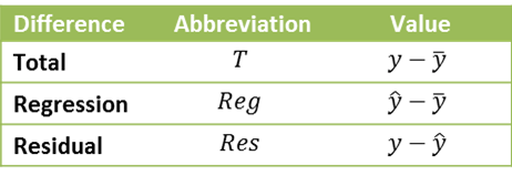
The Residual is the error term of Definition 1. We also define the degrees of freedom df_T, df_Reg, df_Res, the sum of squares SS_T, SS_Reg, SS_Res and the mean squares MS_T, MS_Reg, MS_Res as follows:

Property 1:

Observation: SS_T is the total variability of y (e.g. the variability of life expectancy in Example 1 of One Sample Hypothesis Testing for Correlation). SS_Reg represents the variability of y that can be explained by the regression model (i.e. the variability in life expectancy that can be explained by the number of cigarettes smoked), and so by Property 1, SS_Res expresses the variability of y that can’t be explained by the regression model.

Thus SS_Reg/SS_T represents the percentage of the variability of y that can be explained by the regression model. It turns out that this is equal to the coefficient of determination.

Property 2:

Property 3:

Observation: Note that for a sample size of 100, a correlation coefficient as low as .197 will result in the null hypothesis that the population correlation coefficient is 0 being rejected (per Theorem 1 of One Sample Hypothesis Testing for Correlation). But when the correlation coefficient r = .197, then r² = .039, which means that model variance SS_Reg is less than 4% of the total variance SS_T which is quite a small association indeed. Whereas this effect is “significant”, it certainly isn’t very “large”.

Observation: From Property 2, we see that the coefficient of determination r² is a measure of the accuracy of the predication of the linear regression model. r² has a value between 0 and 1, with 1 indicating a perfect fit between the linear regression model and the data.

Property 4:

Definition 3:  The standard error of the estimate is defined as

Observation: The second assertion in Property 4 can be restated as

For large samples  ≈ 1 and so

Note that if r = .5, then

which indicates that the standard error of the estimate is still 86.6% of the standard error that doesn’t factor in any information about x; i.e. having information about x only reduces the error by 13.4%. Even if r = .9, then s_y.x = .436·s_y, which indicates that information about x reduces the standard error (with no information about x) by only a little over 50%.

Property 5:

a)  The sums of the y values is equal to the sum of the ŷ values; i.e.  = 

b)  The mean of the y values and ŷ values are equal; i.e. ȳ = the mean of the ŷ_i

c)  The sums of the error terms is 0; i.e.  = 0

d)  The correlation coefficient of x with ŷ is sign(b); i.e. r_xŷ = sign(r_xy)

e)  The correlation coefficient of y with ŷ is the absolute value of the correlation coefficient of x with y; i.e.  = ||

f)  The coefficient of determination of y with ŷ is the same as the correlation coefficient of x with y; i.e.  =